Deconstructing Dremel: Google’s Tool For Interactive Analysis of Web-Scale Datasets

Disclaimer: This blog post discusses the paper "Dremel: Interactive Analysis of Web-Scale Datasets" by Sergey Melnik, Andrey Gubarev, Jing Jing Long, Geoffrey Romer, Shiva Shivakumar, Matt Tolton, and Theo Vassilakis. Any formal definitions, problem statement descriptions, examples, and results mentioned in this post are from the original paper, unless otherwise stated. The comments made here are my own and do not reflect the views of the authors.

As part of a recent technical presentation, I gave a talk on the paper “Dremel: Interactive Analysis of Web-Scale Datasets”. Since I’m mainly involved in the AI/ML field, where research moves quickly, I found it quite interesting that a 2010 paper is still relevant today, years after its publication, and even more years after it was implemented at Google in 2006. So I decided to write this blog post about it, diving into its key details and findings.

Motivation

Dremel was first published in 2010 at the VLDB Conference. Conceived at Google, initially as a part-time 20% project [4], and it is still being used today in BigQuery, Google’s data warehouse.

Dremel became popular because it enabled interactive queries on large, multi-terabyte datasets, using familiar SQL syntax, at a time when this was considered impossible. Dremel’s enduring impact was recognized in 2020 when it received the VLDB Test of Time Award.

For the rest of this blog post, let’s consider the following working example as we dive into the inner workings of Dremel. Storage has become cheaper, so the amount of data we can keep has exploded, and with large amounts of data comes the need -or maybe better, the desire- to perform interactive large-scale data analysis.

Let’s assume we have a large dataset of a trillion product pages. Each product page contains a number of suggestions for other similar products as well as the most frequently purchased products. Additionally, let’s say we track the location each product page targets, keeping information such as the language code and country.

Now, suppose we wanted to determine how many of the products target the US market by aggregating the location information. At that time (in Google) we would probably have to write a complicated MapReduce [2] batch job, probably in Sawzall, a language Google introduced to make writing MapReduce jobs easier. Then, we would have to wait a couple of hours for the query to execute. If we then wanted to compare that number to the number of pages targeting the UK market, we would have to repeat the process and wait another hour.

This example highlights the need for business users to have queries that run at interactive speeds, taking seconds (or maybe minutes) to execute, instead of hours. That’s exactly what Dremel did back then.

Ingredients

Dremel has four main ingredients:

• A storage model optimized for analytical (aggregation) queries.
• A data model that supports nested semi-structured data, as opposed to flat, neatly stored relational data.
• An SQL-like query language.
• A query-execution model that can scale across servers.

We’ll go through each of these in the following sections.

Storage Model

When Dremel was introduced, row-oriented storage was the de facto choice for large-scale data processing. This may be because most systems were optimized for OLTP workloads, which frequently involved reading or writing entire rows.

In row-oriented storage, data is stored on disk row by row, and all records of a field are kept together. This means that, even if one cares about the value of a single field across records (which is common in aggregation queries run by data analysts), one would still have to load the entire record into memory before accessing that field. Figure 1 below provides an example.

Figure 1: Row-oriented storage. Even if we only care about the country information (yellow boxes), we’d still have to load the full records to memory to be able to read that information. Based on [1].

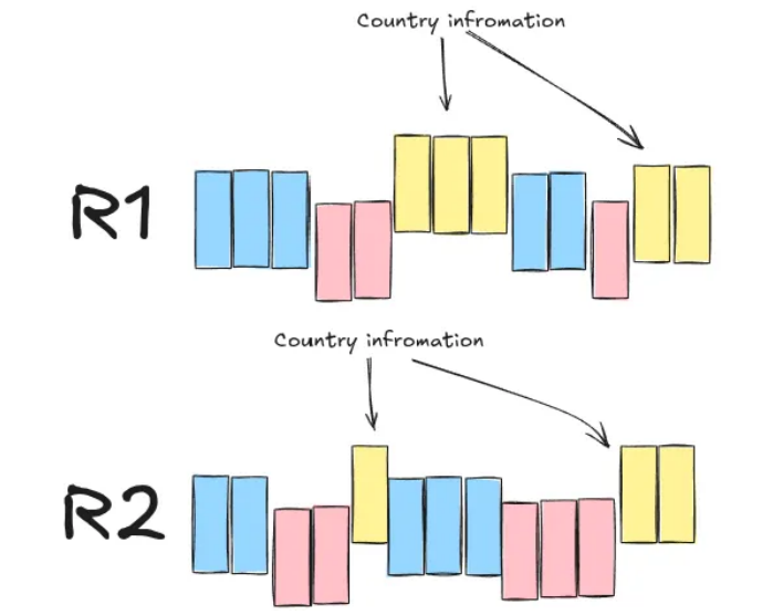
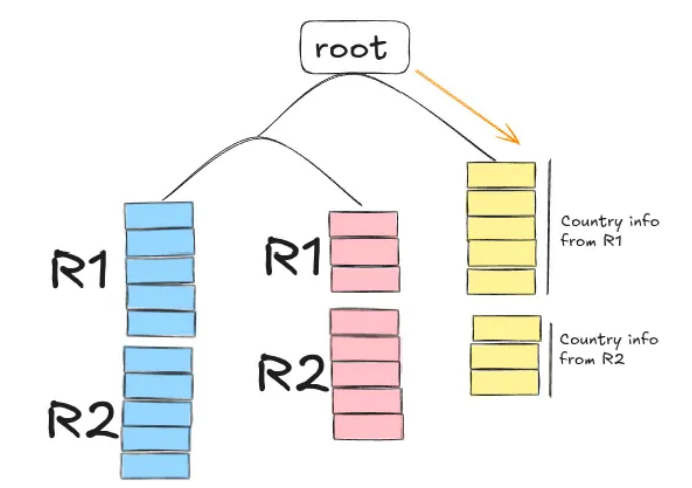
Instead, the Dremel developers opted for column-oriented storage. With this method, all the values for one field across all records are stored together. This means that in aggregation queries, where we only care about the value of one field across records, we can load only those values into memory, effectively disregarding any useless information present on the other fields. Figure 2 shows an example of records R1 and R2 in column-oriented storage.

Figure 2: Column-oriented storage. Since all the values for a specific field are stored together, we can now only read the information we need without scanning irrelevant fields. In our example, we can only read the Country information (yellow boxes) without ever touching the rest of the fields. Based on [1].

This may not seem significant, but keep in mind that data analysts usually care about the aggregated values (sum, average, etc.) of the records in a database. After all, we’re only human; we can’t draw meaningful conclusions when presented with all the fields of all the records in a database; we need to see the bigger picture.

Data Model

The data model is what defines how data is structured and represented in memory.

The web data Dremel primarily targets do not naturally fall under the relational, neatly structured model used in traditional databases. Instead, they are naturally nested, and thus, a data model that can handle nested data was preferred.

Figure 3 below shows an example schema of a nested record representation of our “Product Pages” running example.

Figure 3: Example of a nested schema representing a Product Page from our running example.

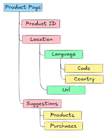
Google’s open-source data serialization format, called Protocol Buffers, naturally supports nested data. It is also strongly typed and offers a compact and efficient data representation in binary format. Additionally, it can easily be extended over time, making it easy to maintain.

Below is an example of a (simplified) schema in Protocol Buffers, for our “Product Pages” running example:

message ProductPage{
    required int 64 ProductId;
    optional group Suggestions{
        repeated string ProductId;
        repeated string PurchasesId;
    }
    repeated group Location{
            repeated group Language{
                required string Code;
                optional string Country;
            }
        optional string Url;
    }
}

This schema includes the following type of fields:

• required fields that must be present in every record
• optional fields that may or may not be present
• repeated fields that can consist of one or more values in the form of a list

It’s important to keep in mind for later that optional and repeated fields can be omitted.

An example of a record that follows our schema definition is:

ProductID: 1
Suggestions
    ProductId: 123
    ProductId: 422
    ProductId: 1200
Location
    Language
        Code: UK
    Language
        Code: US
        Country: United States
    Url: "www.somefancyname.com"

Lossless Representation

Here’s a challenge for you. Let’s say you manage to split the data into a column- oriented format. Now you can easily load only the necessary fields into memory when running aggregation queries. But how would you reconstruct the data to retrieve the original records? Note that some fields may be missing from one record but be present in another, and some fields may appear multiple times in one record but only once in another. In short, we need a way to be able to reconstruct the original records without losing information.

A heads-up before we continue: This next chapter is going to be a bit involved. If you don’t want to know the details of how the Dremel developers offer a lossless representation of the data, feel free to skip it and go directly to the next chapter, which is about Dremel’s SQL-like query language and query execution mechanism.

To enable lossless representation, the authors keep track of three pieces of information: a field’s value along with two integer values representing the repetition, and the definition level of each value. I’ll give the authors’ definitions of these numbers verbatim from the paper [1]:

• Repetition level: this value indicates at which repeated field in a field’s full path, the value has already repeated.
  Note that, by definition, if it is the first time we encounter a field, then the repetition number will be zero. This is later used as a signal that we’re starting a new field, not encountered before.
• Definition level: this value indicates how many fields in a value’s full path that could be undefined (because they are optional or repeated) are actually present

Repetition Level Calculation

To get a better understanding, let’s calculate both the repetition and definition levels for the Code field in these two records:

    Record 1:
        ProductID: 1
        Suggestions
            ProductId: 123
            ProductId: 422
            ProductId: 1200
        Location
            Language
                Code: UK
            Language
                Code: US
                Country: United States
        Location
            Url: "www.somefancyname.com"

    Record 2:
        ProductID: 2
        Suggestions:
            PurchaseId: 1
            PurchaseId: 12
        Location
            Language
                Code: ES

The Code values we care about are: UK, US, and ES. The first two appear in record 1, and the latter appears in record 2. The full path for the code values is Location.Language.Code, and the first value we encounter is UK, so by definition it has a repetition level of 0:

• UK: repetition level = 0

The next value we encounter is US. As the definition states, let’s check at which repeated field in the field’s path that value is repeated. The value is repeated under the second repeated field Language, thus the repetition level for this value is equal to 2:

• US: repetition level = 2

Finally, there is a new Location entry in record one, but there is no Language.Code defined for this, so we’ll leave it as NULL. This field repeats under Location which is the first repeated field in the Location.Language.Code path, so we’ll also track:

• NULL: repetition level = 1

Now let’s move to the second entry, since it’s the first time in that entry that we encounter Location.Language.Code, we’ll append it with repetition level equal to 0:

• ES: repetition level = 0

Note that the order by which we keep the values in memory actually matters, we should encounter ES after we finish processing all the values of record 1.

In summary, the repetition levels for each value are:

Location.Language.Code	Repetition level
UK	0
US	2
NULL	1
ES	0

Definition Level Calculation

Now, let’s calculate the definition level for the same fields. Admittedly, this is a bit easier to calculate.

The full path of the values in the first record is Location.Language.Code. The path contains two fields that can be omitted Location and Language and since both are present, the definition level for the UK and US entries is 2. Then there for the second occurrence in the first record, only Location is defined (there’s no Language) so the definition level is 1.

Notice that when the definition level is less than the maximum possible value, it means that the value for that entry is NULL .

For the second record with a value ES, similar to UK and US entries, the definition number is equal to 2.

In summary, the repetition and definition levels for the Location.Language.Code field are:

Location.Language.Code	Repetition level	Definition level
UK	0	2
US	2	2
NULL	1	1
ES	0	2

Encoding

After calculating the repetition and definition levels, each column is stored as a set of tables containing its compressed values, as well as its repetition, and definition levels. This information is then used to reconstruct the records.

Record Assembly

The assembly of records is done using a finite state machine (FSM) also known as an automaton. If you’re unfamiliar with this concept, don’t worry. In short, an FSM is a collection of states and transitions between those states. In Dremel, the states are field readers that read information from the value-repetition level-definition level blocks and decide whether to write that value or not. The transition between states is dictated by the repetition level.

A nice thing in this design is that we can reconstruct records only with selected fields, without reading unnecessary information. Under the hood, this is done by only activating specific field readers.

I won’t give an example of reconstructing the entire R1 and R2 records from our running example, because it would be too complicated. Instead, let’s walk through a simpler example. Suppose we want to reconstruct each record with only the ProductId and Location.Language.Code fields. Then our automaton (FSM) would look something like the one in Figure 4 below.

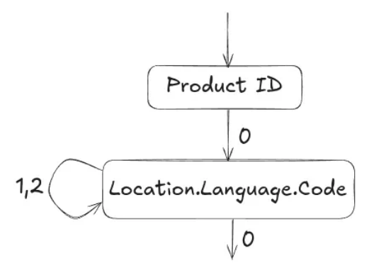
Figure 4: Finite State Machine that reconstructs records containing the ProductId and Location.Language.Code fields. Based on [1].

As a reminder, here are the repetition and definition levels for those fields:

Location.Language.Code	Repetition level	Definition level
UK	0	2
US	2	2
NULL	1	1
ES	0	2

ProductId	Repetition level	Definition level
1	0	0
2	0	0

The first step would be to read the ProductId value and then decide what to read next. Remember that every document has a ProductId value and may contain one or more Location.Language.Code fields.

After reading the first ProductId value and the repetition level 0, the automaton detects that we are starting a new record. So instead of reading the next ProductId value, it switches states to the next field we care about and reads the value UK with repetition level 0.

Again, a repetition level 0 tells us that this is a new record, which has not yet been repeated. So we start a new Location.Language.Code entry under the record with ProductId 1.

So far, our reconstructed entry would look like this:

    > Record 1:
        ProductID: 1
        Location
            Language
                Code: UK

Now, after we moved to state 2, the repetition levels tell us where to jump back in the nesting. So a repetition level of 2 indicates that the repeated field is the second in the full path, the field we are processing. So a new value would mean that we start a new Language field with its code, under the same Location field.

Our reconstructed entry after reading the next value with its repetition level looks like this:

    > Record 1:
        ProductID: 1
        Location
            Language
                Code: UK
            Language
                Code: US

On the other hand, a repetition level of 1 means that the new value would be repeated under the first field in the full path, so it means that we start a new Location field, still under the first record. Since the value we now read is NULL our reconstructed entry would look like this:

    > Record 1:
        ProductID: 1
        Location
            Language
                Code: UK
            Language
                Code: US
        Location
        <-- We have no value for Code so nothing to add here -->

Then we read the value ES with a repetition level of 0. This means we are starting a new record, so we move out of the Location.Language.Code state in our automaton, and start a new record.

Following a similar procedure to the one described above, we end up reconstructing the full records, only for the field we care about.

Query Language & Execution Mechanism

Now let’s switch gears and discuss Dremel’s query language and query execution mechanism.

Dremel used an extended SQL dialect for nested columnar data, which was a significant advantage in 2010. In a retrospective paper published in 2020 [4], the authors mention that SQL was considered “dead” for interactive queries back in 2010. This meant that a lot of alternatives started popping up, including Sawzall (a language designed specifically for MapReduce jobs), C++, and Java.

The main disadvantage of these alternatives was that data analysts were unfamiliar with them, so there was a learning period that had to be spent before they came up to speed. Conversely, almost every data analyst knows SQL. So bringing SQL back into the playing field, specifically for interactive queries, was a big thing.

I won’t spend much time discussing the specifics of Dremel’s SQL-like language, but it’s important to know that it is optimized for columnar nested storage, and it supports features like top-k, joins and nested subqueries. Here’s an example of the syntax:

SELECT ProductId AS Id
    Count(Location.Language.Code) WITHIN Location AS LocationCount
FROM t
WHERE REGEXP(Location.Url, '^www') AND ProductId < 4;

One of the most interesting aspects, in my opinion, is the query execution mechanism of Dremel, which takes the form of a multi-level execution tree (Figure 5).

Figure 5: Multi-level query execution serving tree. Based on [1].

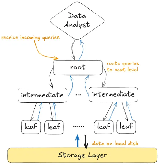
This multi-level serving execution tree is primarily designed for one-pass aggregation queries. Keep in mind that these are the most common type of queries run by data analysts.

In the multi-level serving tree, the root server receives an incoming query from a data analyst, written in Dremel-SQL. Based on the database metadata, the root server rewrites the query and then routes it to the intermediate servers.

For example, if the query was:

SELECT COUNT(*) FROM T

The root server would check for which parts of T each intermediate server is responsible for, and would rewrite the query as:

SELECT COUNT(*) FROM T_i

where T_i is the part of T that the intermediate server i is responsible for. The same procedure occurs for each intermediate server until we reach the leaf nodes that are communicate with the storage layer.

The leaf nodes would be the ones that calculate the result and backward propagate them to the intermediate servers. The intermediate servers then aggregate and backward propagate the results upward, until we reach the root server. Finally, the root server communicates the final result back to the data analyst.

Conclusion

That concludes the behind-the-scenes workings of Dremel that I wanted to share in this post. Be sure to check the official paper[1] for a detailed discussion of the experiments conducted by the authors, and a discussion of the following:

• How column-oriented storage compares to row-oriented storage when it comes to reading and parsing data from disk.
• How Dremel compares to MapReduce in simple aggregation queries.
• How the topology of the multi-level serving tree affects query execution time.
• How they deal with stragglers by allowing approximate aggregation results.

I hope you enjoyed it!

References

1. Dremel: Interactive Analysis of Web-Scale Datasets, , S.Melnik et al., Proceedings of the VLDB Endowment , 2010
2. MapReduce: simplified data processing on large clusters, , J. Dean & S. Ghemawat, Communications of the ACM , 2008
3. Challenges in Building Large-Scale Information Retrieval Systems, , J. Dean, WSDM Invited Talk , 2009
4. Dremel: A Decade of Interactive SQL Analysis at Web Scale, , S.Melnik et al., Proceedings of the VLDB Endowment , 2020

This post summarizes and comments on concepts presented in "Dremel: Interactive Analysis of Web-Scale Datasets (VLDB 2010)". Figures are recreated for educational purposes.