Is there such thing as too much HPO?

Disclaimer: This blog post discusses the paper "Overtuning in Hyperparameter Optimization" by L. Schneider, B. Bischl, and M. Feurer. Any formal definitions, problem statement descriptions, examples, and results mentioned in this post are from the original paper, unless otherwise stated. The comments made here are my own and do not reflect the views of the authors.

What is overtuning?

Imagine that you are trying to tune the hyperparameters (HPs) of a model you’re working on. Let’s say you spend your time running Random Search [2] or you opt in for a more complicated approach using Bayesian optimization. In the end, you find the HPs that perform best on some metric on your validation set. In the final step, you predict on your test set and you get an estimate of your generalization error.

But what if, during this process, you encountered an HP configuration (HPC) earlier in the trajectory, that would perform better on the test set? In other words, what if you overfit, not on the training process, but on the HPO process? That kind of “overfitting” is what the authors of this paper call overtuning, and it might happen more often than you think. After analyzing several tabular benchmarks (i.e. machine learning problems that offer the full learning curves with training, validation, and test metrics) the authors found that overtuning occurs in about 40% of the runs, though it’s typically mild or negligible. However, in about 10% of the cases a phenomenon they call “severe” overtuning occurs, where all HPO progress is lost and the final HPC performs worse than the initial or default HPC.

Definitions

Before discussing the formal definition of overtuning given by the authors, let’s introduce some notation for readers that may not be so familiar with HPO.

• Budget: This is the total number of HPO iterations we are willing to spend. For example if we decide to run Random Search [2] 400 times, effectively trying 400 different HPC, then the budget, denoted as T in the paper, is equal to 400.
• Incumbent: An incumbent is the HPC that has the best validation performance. It follows that for a budget T, the incumbent will probably be different at different stages of the HPO process. We denote the incumbent at budget \(t\) as \(\lambda_t^*\).

During the HPO process, we end up with a sequence of incumbents that looks like this: \((\lambda_1^*, \lambda_2^*, \ldots, \lambda_T^*)\). According to the authors, overtuning occurs if there exists an HPC \(\lambda_{t'}^*\) with higher validation error, but lower test error than the final incumbent \(\lambda_T^*\).

Mathematically, the authors define it as \(ot_t(\lambda_1, \ldots \lambda_{t}, \ldots \lambda_T) = \text{test}(\lambda_t^*) - \min_{\lambda_{t'}^* \in \{\lambda_1^*, \ldots, \lambda_t^*\}} \text{test}(\lambda_{t'}^*)\)

If this quantity is positive, it means that the test of the final incumbent \(\lambda_t^*\) is greater than the minimum test error of a configuration that was previously the incumbent. As a note, \(\lambda_t^*\) was selected based on its validation error.

In order to compare HPO runs from different benchmarks that use different metrics, and, thus, different scales for the test and validation errors, the authors also define relative overtuning as

\[\tilde{ot}_t(\lambda_1, \ldots \lambda_{t}, \ldots \lambda_T) = \frac{ot_t(\lambda_1, \ldots \lambda_{t}, \ldots \lambda_T)}{\text{test}(\lambda_1^*) - \min_{\lambda_{t'}^* \in \{\lambda_1^*, \ldots, \lambda_t^*\}} \text{test}(\lambda_{t'}^*)}\]

On this definition \(\lambda_1^*\) is either the first configuration attempted, or the default configuration. If the relative overtuning is zero, then there is no overtuning; that is, the incumbent that performs best on the validation set, is also the one that performs best on the test set. This is the best case scenario. If the relative overtuning is greater than zero, for example 0.5, half of the improvement in the test performance that was gained during the HPO process, has been lost again due to overtuning. Finally, if relative overtuning is greater than 1, it means that the HPO process ended up with a configuration that performs worse than the initial or default configuration attempted.

The authors also discuss related concepts like meta-overfitting and test regret, but their main focus here is overtuning. For simplicity, I won’t go into those other terms, but the paper carefully separates them.

I think this is a very interesting definition, that opens up further discussion possibilities in the HPO process itself. However, note that we can’t use this definition to combat overtuning itself during the HPO process, since computing it requires knowledge of the test set. This would defeat the purpose of having a test set in the first place. Instead, the authors use overtuning to analyze past HPO runs, using benchmarks that provide the full learning curves, to better understand when and why tuning can sometimes hurt generalization performance.

Another interesting point, which the authors also discuss, is that overtuning and relative overtuning are not designed as measures to compare different HPO methods. For instance, if random search has lower relative overtuning than Bayesian optimization, that does not mean that you should use random search. The authors additionally provide a helpful numerical example in which an HPO method, e.g. method A may evaluate only a single configuration that achieves a validation error of 0.3 and a test error of 0.35. Based on the definition we discussed above, this method would exhibit no overtuning. Next they consider method B, which evaluates 10 different HP configurations with the final best HP configuration achieving a validation error of 0.18 and a test error of 0.22. Now, assuming method B also had an HP configuration that, if chosen, would exhibit a test error of 0.2. This then means that method B has an overtuning of 0.02. But notice that it leads to better test error overall. This shows that overtuning doesn’t necessarily mean the final result is bad, but rather that the HPO process could have been more efficient.

How often it happens?

After providing the necessary definitions, the authors conducted an exploratory analysis of seven large-scale studies (FCNet[3], LCBench[4], WDTB[5], TabZilla[6], TabRepo[7], reshuffling[8], and PD1[9]) with publicly available HPO trajectories and learning curves. They explore how often and to what extent overtuning occurs.

Figure 1, which is also from the paper, sums up their main findings

Figure 1: ECDF of relative overtuning for the seven large-scale studies [1].

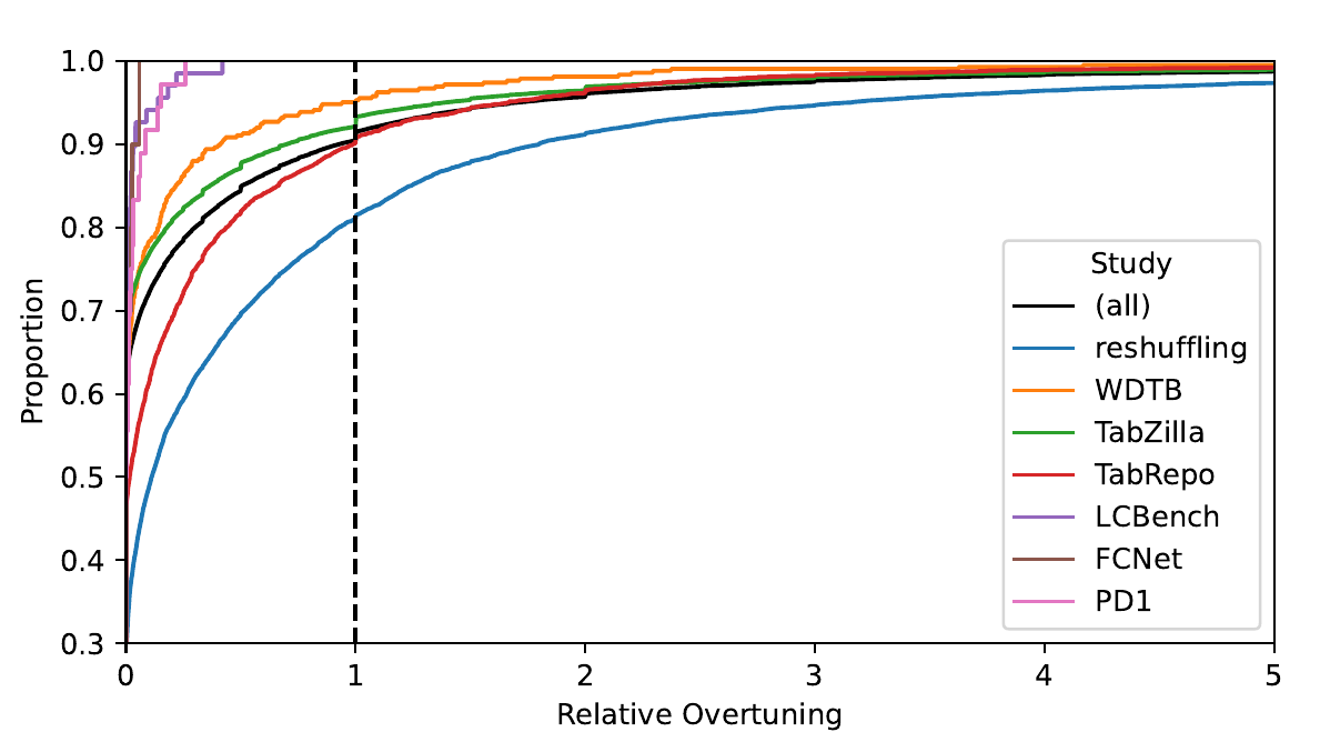
The figure illustrates the empirical cumulative distribution function (ECDF) of relative overtuning across the seven large-scale studies. It also includes the aggregated results across all studies (black line with the label “all”). The way to read this plot is the following: for each value on the x-axis, the corresponding value of the y-axis gives the fraction (%) of HPO runs that have relative overtuning less than or equal to the x-axis value. For instance, at x=0, the aggregated results line (black) has a y-value of approximately 0.6. This means that approximately 60% of the runs exhibit no overtuning. Another example is at x=0.5, where the y-value is approximately 0.84. This means that approximately 84% of the runs exhibit relative overtuning less than or equal to 0.5.

An interesting point is the y-value for x=1. This is what the authors call “severe” overtuning, i.e., relative overtuning greater than one. This occurs in about 10% of the runs. As it can be seen from the plot, there is significant variance between different benchmarks. For a detailed analysis of each, see the paper.

What are possible causes?

To model the possible causes, the authors performed an exploratory analysis of the reshuffling [8] data. They focused mainly on the following factors:

• budget
• performance metric
• machine learning algorithm
• resampling strategy (i.e., how the data is split into training, validation, and test sets)
• dataset size

They use a generalized linear mixed-effects model (GLMM) to predict overtuning likelihood with different settings, and a linear mixed-effects model (LMM) to model how severe relative overtuning can be for different settings.

In a nutshell, a GLMM considers a linear combination of some fixed factors, along with some random coefficients for factors that may vary across different groups, such as dataset or seed. The output of the GLMM is then passed through a link function to yield a probability between 0 and 1. The LMM is similar, but it assumes that the outcome is Gaussian and does not use a link function. A simplified GLMM model that could be used to predict the probability of overtuning might look something like this:

\[\text{logit}(p_{ijk}) = \beta_0 + \beta_1 \,\text{budget}_{ijk} + \beta_2 \,\text{budget}_{ijk}^2 \\ + \sum_{m}\gamma_m \,\text{Metric}_{m,ijk} \\ + \sum_{c}\delta_c \,\text{Classifier}_{c,ijk} \\ + \sum_{r}\rho_r \,\text{Resampling}_{r,ijk} \\ + \sum_{s}\eta_s \,\text{Size}_{s,ijk} \\ + u_{\text{data}[i]} + v_{\text{seed}[j]}, \\\]

where the random effects are modeled as

\[u_{\text{data}[i]} \sim \mathcal{N}(0,\sigma^2_{\text{data}}), \quad v_{\text{seed}[j]} \sim \mathcal{N}(0,\sigma^2_{\text{seed}}).\]

In this equation, the choice of performance metric, machine learning algorithm, resampling strategy, and dataset size are one-hot encoded.

Their results are depicted on the following tables

Table 1: GLMM coefficients for prediction of overtuning from [1].

Table 2: LMM coefficients for prediction of relative overtuning from [1].

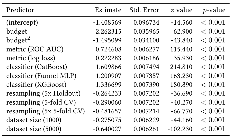
The way to read these tables is that the higher the value in the “Estimate” column, the higher the likelihood of overtuning due to that factor compared to the default factor. For instance, in the GLMM that predicts the presence or not of overtuning (Table 1), the ROC AUC metric has a factor of 0.724608, while the log-loss metric has a factor of 0.222283. This means that both metrics increase the odds of overtuning, however ROC AUC increased the odds more strongly than the default metric, which was accuracy. Log-loss also raised the odds but to a smaller extent.

The authors also highlight another interesting aspect, that longer tuning (i.e, a higher budget) generally increases the odds of non-zero overtuning; however the quadratic term of \(\text{budget}^2\) is negatively associated with non-zero overtuning. As the authors mention, this probably indicates that after a point the effect levels off. In other words, more iterations help up to a point, after which the gains diminish.

Interestingly enough, all classifiers are associated positively with non-zero overtuning compared to the default, which in this case was ElasticNet. Finally, as expected, dataset size is negatively associated. The default value for dataset size was 500.

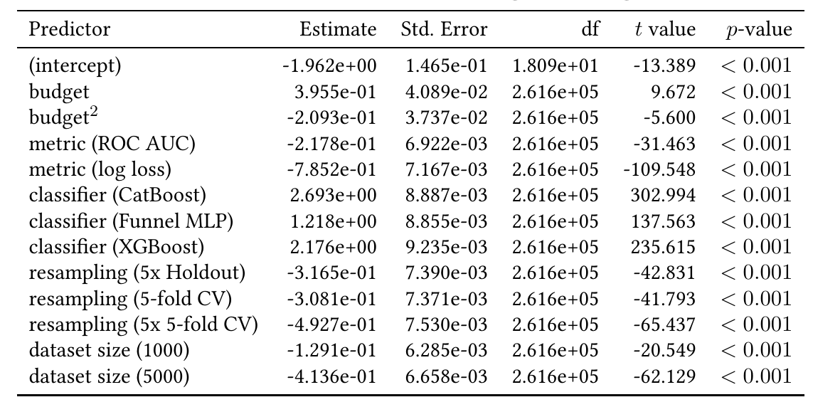
The results are somewhat similar for the LMM case (Table 2).

Note that these effects were observed in the analyzed benchmarks and may vary across datasets and resampling strategies.

What can we do about it?

Although this was not the paper’s main focus, the authors mention several ways to reduce overtuning: using a more robust resampling strategy, adding regularization, or using early stopping. They also discuss more advanced techniques such as reshuffling validation splits, ways of choosing incumbents more conservatively, or using Bayesian optimization to smooth noisy validation scores. Not all of these are practical in every setting, but together they show that overtuning can be mitigated.

Conclusion

That’s all I wanted to share in this blog post. I found the work exciting, and I believe it opens up new discussion points both in the fields of hyperparameter optimization and automated machine learning. I hope you enjoyed it.

For more details and an in-depth analysis, I strongly suggest reading the original paper here. All the code used by the authors to perform the analyses mentioned in the paper has been released here.

Till next time.

References

1. Overtuning in Hyperparameter Optimization , Schneider, L., Bischl, B., Feurer, M., AutoML 2025 Methods Track , 2025
2. Random Search for Hyper-Parameter Optimization , Bergstra, J. and Bengio, Y, Journal of Machine Learning Research , 2012
3. Tabular benchmarks for Joint Architecture and Hyperparameter optimization. , Klein, A. and Hutter, F., , 2019
4. Auto-Pytorch: Multi-fidelity metalearning for efficient and robust AutoDL. , Zimmer, L., Lindauer, M., and Hutter, F., IEEE Transactions on Pattern Analysis and Machine Intelligence , 2021
5. Why do tree-based models still outperform deep learning on typical tabular data? Grinsztajn, L., Oyallon, E., and Varoquaux, G., Proceedings of the 35th International Conference on Advances in Neural Information Processing Systems (NeurIPS’22). , 2022
6. When do neural nets outperform boosted trees on tabular data? , McElfresh, D., Khandagale, S., Valverde, J., Prasad C, V., Ramakrishnan, G., Goldblum, M., and White, C., 37th Conference on Neural Information Processing Systems Datasets and Benchmarks Track , 2023
7. TabRepo: A large scale repository of tabular model evaluations and its AutoML applications. , Salinas, D. and Erickson, N. Proceedings of the Third International Conference on Automated Machine Learning , 2024
8. Reshuffling resampling splits can improve generalization of hyperparameter optimization. , Nagler, T., Schneider, L., Bischl, B., and Feurer, M. Proceedings of the 37th International Conference on Advances in Neural Information Processing Systems (NeurIPS’24). , 2024
9. Pre-trained Gaussian processes for Bayesian optimization. , Wang, Z., Dahl, G. E., Swersky, K., Lee, C., Nado, Z., Gilmer, J., Snoek, J., and Ghahramani, Z., Journal of Machine Learning Research, Vol. 25 , 2024